New Columns from Old: Math, np.where and cut
Math between columns makes a new column for every row at once, np.where picks one of two values for each row from a True or False column, pd.cut sorts numbers into labeled bands such as budget, mid and premium, and apply runs a function of your own on every value, more slowly than whole-column math.
Journeyman · Python · Updated
After this lesson you can
- Add a column calculated from other columns with whole-column math, and np.where for an either-or value
- Group numbers into labeled bands with pd.cut, choosing the edges and which side each edge belongs to
- Use apply with a function or a lambda, and explain why whole-column math is faster than apply
Key takeaways
- Math between columns, such as products["price"] * products["stock"], works on every row at once and makes a new column.
- np.where(condition, value_if_true, value_if_false) gives each row one of two values, such as a sale price or the normal price.
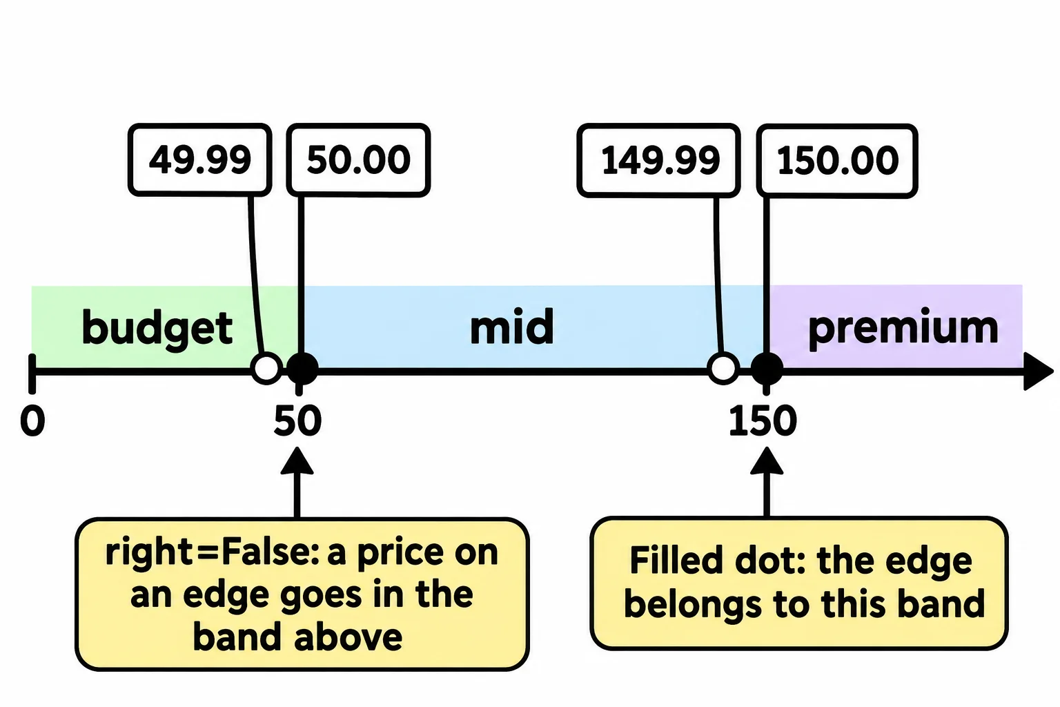
- pd.cut sorts numbers into labeled bands. right=False puts a value that sits exactly on an edge, such as 50, into the band above it.
- apply runs a function, or a lambda (a small function with no name), on every value, one at a time.
- Whole-column math is much faster than apply, so use apply only when no column operation does the job.
The numbers you need are often not in the table. A store owner asks how much money is sitting on the shelves, but the catalog has a price and a stock count, not their product. A sale needs a sale price for some products and the normal price for the rest. A report wants products grouped as budget, mid-range and premium. Each answer is a new column worked out from the columns you have, and it's the step between "the data we got" and "the question we were asked".
The example is Trailhead Outfitters' catalog, products.csv: 300 outdoor gear products with their product name, category, price, stock, on_sale (True or False), weight_oz and more. The catalog is our own made-up data.
Math on whole columns
Multiplying two columns multiplies them row by row, the first price by the first stock, the second by the second, all 300 at once. Assigning the result to a new name adds it as a column:
import pandas as pd
import numpy as np

products = pd.read_csv("products.csv")
products["stock_value"] = products["price"] * products["stock"]
products[["product", "price", "stock", "stock_value"]].head(3)
                   product   price  stock  stock_value
0          Mesa Glide Tent  182.99     18      3293.82
1         Basalt Trek Tent  231.99     38      8815.62
2  Mesa Glide Sleeping Bag  113.99     10      1139.90
VS Code draws the table as a grid; this lesson shows it as pandas prints it as text. A column and a single number work too, so products["weight_oz"] / 16 gives every weight in pounds. The line import numpy as np (read "n p", NumPy's short name) loads NumPy, which comes with pandas; the next section uses it, and NumPy: The Engine Under pandas explains what it is.
Either-or values: np.where
This weekend, products on sale are 20% off. Each row needs one of two values: the price times 0.8 if on_sale is True, the price as it is if not. That's np.where: a condition, the value where it's True, and the value where it's False.
products["sale_price"] = np.where(products["on_sale"], (products["price"] * 0.8).round(2), products["price"])
products[["product", "price", "on_sale", "sale_price"]].iloc[3:6]
             product   price  on_sale  sale_price
3  Cascade Trek Tent  176.99    False      176.99
4  Aspen Trek Jacket   58.99     True       47.19
5   Alpine Pro Boots   67.99    False       67.99
Read it as "where on sale, 80% of the price, otherwise the price". The condition can be any mask, such as products["stock"] == 0.
Bands: pd.cut
The store sorts products into three bands: budget under $50, mid from $50 up to $150, premium $150 and up. pd.cut takes the numbers, the edges of the bands (bins), and a name for each band:
products["price_band"] = pd.cut(
    products["price"],
    bins=[0, 50, 150, float("inf")],
    labels=["budget", "mid", "premium"],
    right=False,
)
products["price_band"].value_counts()
price_band
premium    178
mid        106
budget      16
Name: count, dtype: int64
float("inf") is infinity, so the last band has no top. Four edges make three bands, so there's one label fewer than edges.
The edges need one decision: a price of exactly 50, is it budget or mid? By default, pd.cut puts an edge value in the band below it (each band includes its right edge). right=False puts it in the band above, so 49.99 is budget, 50.00 is mid and 150.00 is premium, which is what "from $50" means. Your textbook may call this binning a numeric column.
Your own rule: apply and lambda
Sometimes the rule is easier to write as a function. Here, a product under 16 ounces fits in a pocket, under 48 in a pack, and anything heavier rides in the car. apply runs a function on every value of a column and collects the answers:
def carry_size(weight):
    if weight < 16:
        return "pocket"
    if weight < 48:
        return "pack"
    return "car"

products["carry"] = products["weight_oz"].apply(carry_size)
products["carry"].value_counts()
carry
pack      152
car       113
pocket     35
Name: count, dtype: int64
apply is given the function's name, carry_size, with no parentheses: pandas calls it once for each value. For a one-line rule, a lambda (a small function with no name) saves writing a def. lambda price: round(price * 1.07, 2) is read "given a price, give back the price times 1.07, rounded to cents", the price with 7% sales tax:
products["price_with_tax"] = products["price"].apply(lambda price: round(price * 1.07, 2))
products[["product", "price", "price_with_tax"]].head(2)
            product   price  price_with_tax
0   Mesa Glide Tent  182.99          195.80
1  Basalt Trek Tent  231.99          248.23
That works, and so does (products["price"] * 1.07).round(2), with the same answers. Choose the second. apply calls a Python function once per row: 300 calls here, a million calls on a million rows. Whole-column math hands the whole column to NumPy, which does the arithmetic in one fast loop. On a million prices, the whole-column version is dozens of times faster. Reach for apply when the rule needs real Python, like carry_size's ifs, and for whole-column math, np.where or pd.cut whenever they can do the job.
Check yourself
2 questions to try on the lesson page.
So what
New columns turn the data you have into the numbers you were asked for: whole-column math and np.where for amounts, pd.cut for bands, and apply for the rules that need a function of your own.