Your First Chart
A bar chart shows at a glance what a column of numbers makes you read digit by digit, and matplotlib draws one in a few lines, with a title and axis labels so the reader knows what it shows, saved as an image file with savefig.
Apprentice · Python · Updated
After this lesson you can
- Draw a bar chart with matplotlib, using fig, ax = plt.subplots() and ax.bar, and give it a title and axis labels
- Tell a Figure from an Axes, and save a chart as an image file with fig.savefig
Key takeaways
- A chart shows at a glance what a column of numbers makes you read digit by digit, and a bar chart compares amounts across groups, such as sales by store.
- fig, ax = plt.subplots() makes a Figure, the whole image, and an Axes, the one chart drawn on it.
- ax.bar(labels, heights) draws the bars, and set_title, set_xlabel and set_ylabel say what the chart shows and in what units.
- fig.savefig("sales-by-store.png") saves the chart as an image file, and the ending of the file's name picks the type.
The numbers from an analysis end up in front of people: a manager at Monday's meeting, a class reading your lab report, a club looking at this year's sign-ups. Most of them won't read a table of numbers, but they will look at a chart. This lesson draws your first one with matplotlib, the package most Python charts are made with, and saves it as a picture you can put in a report or a slide.
The example is Bean Street Coffee, a small chain with three stores, and its sales for the first week of October in sales.csv, the file from Your First pandas Table: one row for each store on each day, with the date, the store, the cups sold and the sales in dollars.
Three numbers in a meeting
pandas already totals the week by store:
import pandas as pd

week = pd.read_csv("sales.csv")
totals = week.groupby("store")["sales"].sum()
print(totals)
store
Campus      6562
Downtown    8227
Harbor      6718
Name: sales, dtype: int64
Rosa, the owner, wants to show these at the staff meeting. Read them as the staff would: is Harbor ahead of Campus, and by how much? Is Downtown far ahead, or a little? The answers are there, but each one takes reading and comparing digits. A bar chart draws each amount as a bar whose height is the amount, so the comparison is something you see in a second: the tallest bar sold the most.
A Figure and an Axes
Picture a sheet of paper with one chart drawn on it. In matplotlib the sheet is the Figure, the whole image that gets saved, and the chart is the Axes: the area with the bars and the two lines they're measured against. (Axes is the word matplotlib uses even for one chart.) One line makes both:
import matplotlib.pyplot as plt
import pandas as pd

week = pd.read_csv("sales.csv")
totals = week.groupby("store")["sales"].sum()

fig, ax = plt.subplots()
ax.bar(totals.index, totals.values)
fig.savefig("sales-by-store.png")
print("Saved sales-by-store.png")
Saved sales-by-store.png
import matplotlib.pyplot as plt brings in matplotlib's drawing tools under the short name plt. plt.subplots() hands back two things, the Figure and the Axes, and fig, ax = ... unpacks them into two variables, as Tuples and Unpacking shows. ax.bar(labels, heights) draws one bar for each label: here the store names, totals.index, and the totals, totals.values. You draw on the Axes and save the Figure.
Open sales-by-store.png in VS Code and you'll find three blue bars with the stores' names under them, and nothing else. What are the numbers up the side: dollars, cups, customers? Which week? A chart with no words leaves the reader to guess.
A title and axis labels
Three more lines give the chart its words. The x-axis runs along the bottom and the y-axis up the side:
import matplotlib.pyplot as plt
import pandas as pd

week = pd.read_csv("sales.csv")
totals = week.groupby("store")["sales"].sum()

fig, ax = plt.subplots()
ax.bar(totals.index, totals.values)
ax.set_title("Bean Street Coffee: Sales by Store")
ax.set_xlabel("Store")
ax.set_ylabel("Sales ($)")
fig.savefig("sales-by-store.png")
print("Saved sales-by-store.png")
Saved sales-by-store.png
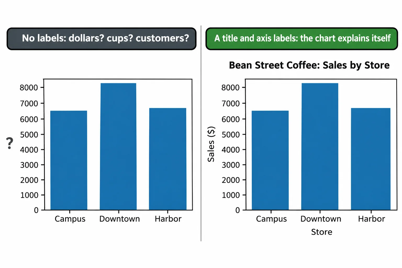
set_title puts a heading over the chart, and set_xlabel and set_ylabel name each axis. Put the unit in the label, ($) here, so nobody has to ask. Now the chart answers Rosa's question by itself: Downtown's bar is the tallest, and Harbor's is a little taller than Campus's.
Saving it: savefig
fig.savefig("sales-by-store.png") writes the Figure to a file in the folder the script runs in, and running the script again replaces it. The ending of the name picks the kind of file: .png for a picture to put in a slide or a web page, .pdf or .svg for one that stays sharp at any size. While you're trying things out, plt.show() opens the chart in a window instead; the script waits there until you close it, so call savefig first.
Where to go from here
That's data analysis in an hour: a table, a few questions, and a chart someone else can read. Real data is messier than Bean Street's week. It has blank cells, prices typed as text and dates in three formats, and the questions get harder: which drinks sell best in the afternoon, and is that changing month to month? Python for Data Analysis is the course that goes further. It works in notebooks, cleans messy data, joins tables, draws line charts, scatter plots and histograms that stay honest, and turns an analysis into a report someone else can follow, and it picks up Bean Street Coffee where this lesson leaves off.
Check yourself
2 questions to try on the lesson page.
So what
A chart with a clear title and labeled axes answers a question at a glance, which is why most analyses end with one.