Honest Axes: Where the Scale Starts
A bar's length is its value, so a bar chart's y-axis starts at zero with ax.set_ylim(bottom=0), because an axis that starts higher makes a small difference look several times bigger; a line chart may zoom in if its label says so, and side-by-side charts share one scale with sharey=True.
Journeyman · Python · Updated
After this lesson you can
- Start a bar chart's y-axis at zero with ax.set_ylim(bottom=0), and explain how a cut-off axis exaggerates a small difference
- Put side-by-side charts on one scale with sharey=True, and say when zooming in on a line chart's axis is fair
Key takeaways
- The eye reads a bar by its length, so a bar chart's y-axis starts at zero. ax.set_ylim(bottom=0) sets it.
- An axis that starts at 60 drew a 1.7-point difference as one bar more than twice as tall as the other.
- A line chart is read by its ups and downs, so it may zoom in on its values, as long as its axis label says where the axis starts.
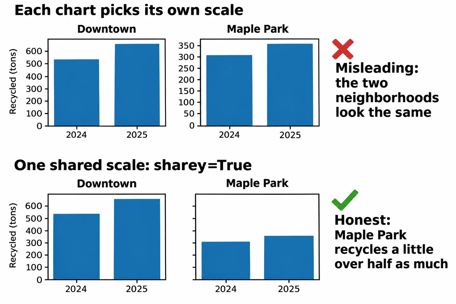
- Two charts side by side are compared by eye, so they share one scale. plt.subplots(1, 2, sharey=True) gives them the same y-axis.
Some charts mislead without a single wrong number. The data is right, the bars are right, and the reader still comes away believing something false, because of where the axis starts. You'll see it in ads, news stories and slides at work, and once you know the trick you can't miss it. This lesson keeps your own charts from doing it, even by accident.
The example is Clearwater City's recycling log, pickups.csv: one row for each of six neighborhoods in each month of 2024 and 2025, with households and households_recycling (how many set out a recycling cart that month) among its columns. Curbside recycling pickup began in January 2025.
Two neighborhoods, one small difference
What share of households recycled in Lakeview and in Oak Hill in 2025? Total the year, then divide:
import matplotlib.pyplot as plt
import pandas as pd

pickups = pd.read_csv("pickups.csv", parse_dates=["month"])
year_2025 = pickups[pickups["month"].dt.year == 2025]
totals = year_2025.groupby("neighborhood")[["households_recycling", "households"]].sum()
rate = (totals["households_recycling"] / totals["households"] * 100).round(1)
two = rate[["Lakeview", "Oak Hill"]]
two
neighborhood
Lakeview    61.2
Oak Hill    62.9
dtype: float64
Close: 61.2% and 62.9%, a difference of 1.7 percentage points. Now draw them the way a newsletter might, with the y-axis set to start at 60. ax.set_ylim (read "set y lim", the y-axis limits) sets where the y-axis starts and ends:
fig, ax = plt.subplots()
ax.bar(two.index, two.values)
ax.set_ylim(60, 63.5)
ax.set_title("Households recycling, 2025")
ax.set_ylabel("Households recycling (%)")
plt.show()
Oak Hill's bar towers over Lakeview's. A reader glancing at it would say Oak Hill recycles more than twice as much. Here's what was drawn:
for name, value in two.items():
    print(f"{name}: {value}%, bar drawn {value - 60:.1f} points tall")
Lakeview: 61.2%, bar drawn 1.2 points tall
Oak Hill: 62.9%, bar drawn 2.9 points tall
Bars start at zero
A bar chart is read by length: a bar twice as long means twice as much. Start the axis at 60 and you cut the same 60 points off every bar, so the bars' lengths stop matching their values. Lakeview's bar shows 1.2 of its 61.2 points, Oak Hill's 2.9 of its 62.9, and the eye compares 1.2 with 2.9. An axis cut off like this is called a truncated axis, and it's the most common way a chart misleads.
The fix is one argument. ax.set_ylim(bottom=0) starts the axis at zero and lets matplotlib choose the top:
fig, ax = plt.subplots()
ax.bar(two.index, two.values)
ax.set_ylim(bottom=0)
ax.set_title("Households recycling, 2025")
ax.set_ylabel("Households recycling (%)")
plt.show()

bottom, top = ax.get_ylim()
print("y-axis starts at:", bottom)
y-axis starts at: 0.0
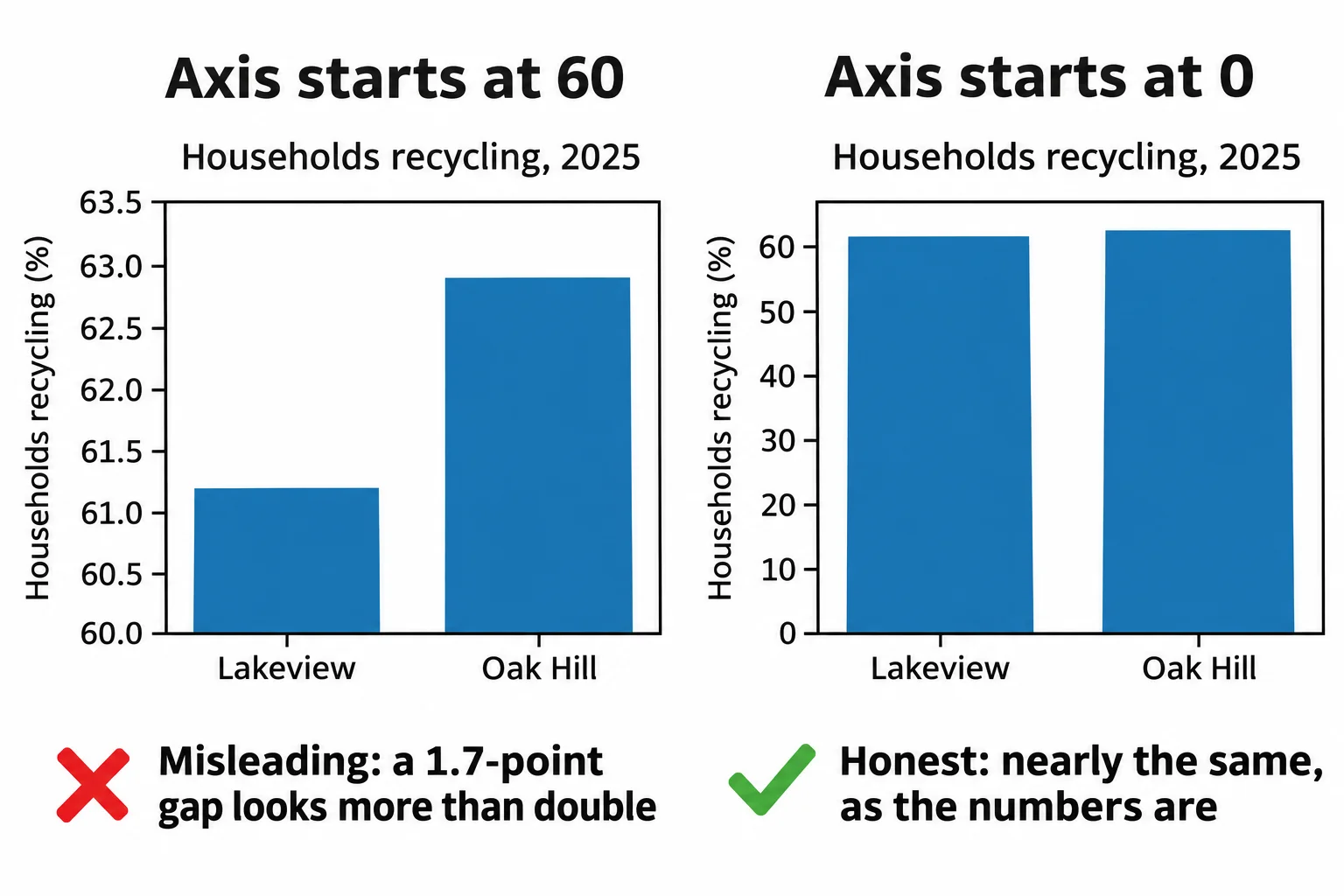
Now the bars are nearly the same height, which is the truth: the two neighborhoods recycle at about the same rate. matplotlib's ax.bar starts at zero on its own; the danger is a set_ylim someone added to "zoom in". When the small difference is the story, say it in words or chart the difference itself.
A line may zoom in, if it says so
A line chart is different. It's read by its ups and downs, not by the length of anything, so zooming in on where the values are can be fair. The city's monthly recycling runs from about 187 to 296 tons, and starting the axis at 150 shows the rise clearly. Say so in the axis label, so nobody reads the bottom of the chart as zero:
monthly = pickups.groupby("month")["tons_recycled"].sum()

fig, ax = plt.subplots()
ax.plot(monthly.index, monthly.values, marker="o")
ax.set_ylim(150, 310)
ax.set_title("Monthly recycling, 2024 to 2025")
ax.set_ylabel("Recycled (tons, axis starts at 150)")
fig.autofmt_xdate()
plt.show()
Side by side on one scale: sharey
Two charts side by side are compared by eye, so they need the same scale. Here are Downtown's and Maple Park's tons for each year, in two charts made by plt.subplots(1, 2), which hands back a Figure and two Axes:
by_year = pickups.groupby(["neighborhood", pickups["month"].dt.year])["tons_recycled"].sum()

fig, (left, right) = plt.subplots(1, 2)
left.bar(["2024", "2025"], by_year["Downtown"].values)
left.set_title("Downtown")
right.bar(["2024", "2025"], by_year["Maple Park"].values)
right.set_title("Maple Park")
left.set_ylabel("Recycled (tons)")
plt.show()

print("Downtown's axis tops out at", round(left.get_ylim()[1]))
print("Maple Park's axis tops out at", round(right.get_ylim()[1]))
Downtown's axis tops out at 684
Maple Park's axis tops out at 374
Each chart chose its own scale, so the bars look the same size, though Downtown recycled almost twice as much. sharey=True gives both charts one y-axis:
fig, (left, right) = plt.subplots(1, 2, sharey=True)
left.bar(["2024", "2025"], by_year["Downtown"].values)
left.set_title("Downtown")
right.bar(["2024", "2025"], by_year["Maple Park"].values)
right.set_title("Maple Park")
left.set_ylabel("Recycled (tons)")
plt.show()

print("Downtown's axis tops out at", round(left.get_ylim()[1]))
print("Maple Park's axis tops out at", round(right.get_ylim()[1]))
Downtown's axis tops out at 684
Maple Park's axis tops out at 684
Check yourself
2 questions to try on the lesson page.
So what
Where an axis starts decides what a reader believes: bars from zero, a zoomed line that says so, and side-by-side charts on one scale keep a true number from telling a false story.