Curves with Polynomial Features
When the label rises and then falls, a straight line misses both ends, but adding a squared copy of a feature lets a linear regression draw a curve; PolynomialFeatures makes those columns, fit on the training rows and used to transform both parts, and a high degree swings wildly at the edges of the data.
Journeyman · AI Basics · Python · Updated
After this lesson you can
- Turn a feature into curve features with PolynomialFeatures, fitting it on the training rows and transforming both parts
- Explain how a squared feature lets a linear model draw a curve, and what a high degree does at the edges of the data
Key takeaways
- A straight line can't follow a label that rises and then falls, such as a harvest that peaks at 30 inches of rain.
- Adding the feature squared as a second column lets a linear regression draw a curve. It's still a linear model, because each column only gets a coefficient.
- PolynomialFeatures makes those columns. Use fit_transform on the training rows and transform on the test rows.
- A higher degree fits the training rows a little better and can swing wildly at the edges of the data and beyond them.
Some things are good only up to a point. A little rain grows apples, too much drowns the roots; a warm day sells more ice cream, a scorching one keeps people home; a little fertilizer helps a lawn, a lot burns it. Whenever more of something helps and then hurts, a straight line gives the wrong answer at both ends, and you'll meet that shape in sales, prices, harvests and sensor readings.
The example is Hilltop Orchard's orchard.csv, from Exercise: Orchard Harvest Models: 200 trees' harvests in pounds of apples, with the rain each tree got that season. Each code block is one notebook cell, run in order: the first one loads the data, and the others use what it made.
A straight line through a hump
Here is the habit from Splitting Data with train_test_split: split first, then fit a line on the training trees.
import pandas as pd
from sklearn.linear_model import LinearRegression
from sklearn.metrics import mean_absolute_error
from sklearn.model_selection import train_test_split
from sklearn.preprocessing import PolynomialFeatures

orchard = pd.read_csv("orchard.csv")
X = orchard[["rainfall_inches"]]
y = orchard["apples_lbs"]
X_train, X_test, y_train, y_test = train_test_split(X, y, test_size=0.2, random_state=42)

line = LinearRegression()
line.fit(X_train, y_train)
print("Pounds per inch of rain:", round(line.coef_[0], 2))
print("Test MAE:", round(mean_absolute_error(y_test, line.predict(X_test)), 1))
Pounds per inch of rain: 0.4
Test MAE: 54.8
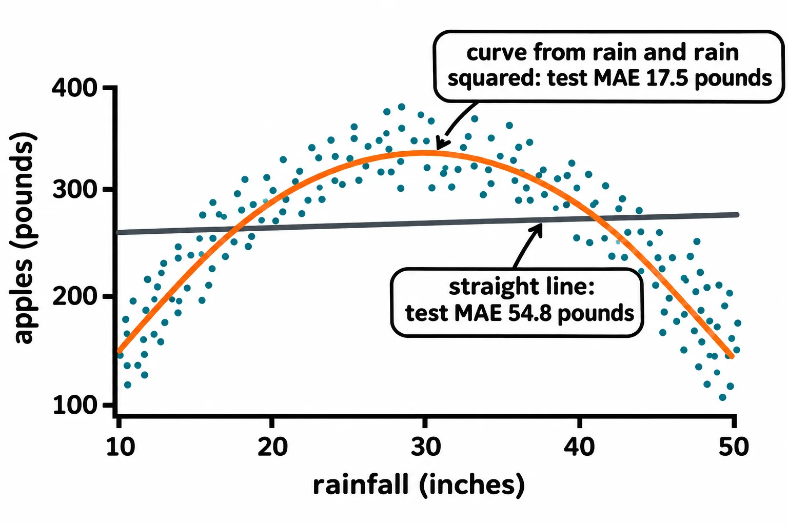
The line says rain barely matters: 0.4 pounds an inch. On the test trees it's off by about 55 pounds on average (Errors and the Mean Absolute Error explains the MAE). Now look at the trees themselves:
for low, high in [(10, 14), (28, 32), (46, 50)]:
    rows = orchard[(orchard["rainfall_inches"] >= low) & (orchard["rainfall_inches"] < high)]
    print(low, "to", high, "inches:", len(rows), "trees,", round(rows["apples_lbs"].mean()), "pounds on average")
10 to 14 inches: 27 trees, 187 pounds on average
28 to 32 inches: 13 trees, 333 pounds on average
46 to 50 inches: 23 trees, 193 pounds on average
Dry trees and soaked trees grew far less than trees with about 30 inches. The harvest rises, peaks and falls. A straight line can only tilt one way, so the best it can do is lie almost flat through the middle and miss both ends.
Adding rain squared
A curve that rises and falls is what you get from a number squared. Give the model a second column, the rainfall squared, and it can learn a curve: the guess becomes the intercept, plus one coefficient times the rain, plus another times the rain squared.
squared_train = X_train.assign(rainfall_squared=X_train["rainfall_inches"] ** 2)
squared_test = X_test.assign(rainfall_squared=X_test["rainfall_inches"] ** 2)

curve = LinearRegression()
curve.fit(squared_train, y_train)
print("Coefficients:", curve.coef_.round(3))
print("Test MAE:", round(mean_absolute_error(y_test, curve.predict(squared_test)), 1))
Coefficients: [27.765 -0.464]
Test MAE: 17.5
** is Python's power operator, read "to the power of": ** 2 squares. The negative coefficient on the squared column bends the curve down at both ends, and the test MAE drops from 54.8 to 17.5 pounds. The seed script planted a peak at 30 inches; multiplied out, its formula has 27 for the rain and −0.45 for the rain squared, and the model came close.
This is still LinearRegression: each column gets one coefficient, added up, exactly as in More Than One Feature. The curve comes from the columns, not from a new kind of model. Statistics classes call this polynomial regression.
PolynomialFeatures makes the columns
Writing squared columns by hand gets tedious with more features. scikit-learn's PolynomialFeatures makes them for you:
poly = PolynomialFeatures(degree=2, include_bias=False)
curve_train = poly.fit_transform(X_train)
curve_test = poly.transform(X_test)
print(poly.get_feature_names_out())
print("Shapes:", curve_train.shape, curve_test.shape)
print(curve_train[:2])
['rainfall_inches' 'rainfall_inches^2']
Shapes: (160, 2) (40, 2)
[[  41.94   1758.9636]
 [  47.55   2261.0025]]
degree=2 means powers up to 2, and ^2 in the names is read "squared". include_bias=False leaves out a column of 1s that LinearRegression's intercept already covers. With two features, degree 2 also adds each one squared and the two multiplied together.
The two calls follow the same habit as the split: fit_transform learns from the training rows and changes them, and transform only changes the test rows, using what was learned. Here, "learned" is only how many columns there are, but later steps learn averages from the data, and the habit keeps the test rows unseen. The result is a plain grid of numbers, an array, so you fit on it as before:
model = LinearRegression()
model.fit(curve_train, y_train)
print("Test MAE:", round(mean_absolute_error(y_test, model.predict(curve_test)), 1))
Test MAE: 17.5
The same 17.5 pounds: the same columns as the hand-made ones.
Higher degrees and the edges
If degree 2 helps, does degree 15 help more? Not here. A high power of 50 inches is a huge number (50 to the 15th power has 26 digits), and the arithmetic loses precision, so this cell first measures rain in tens of inches away from 30, the middle of the range. The curves it can draw are the same; only the numbers are smaller. Scaling Features does this properly later in the course.
def tens_from_30(table):
    return (table - 30) / 10

edges = pd.DataFrame({"rainfall_inches": [8, 30, 50, 52]})
for degree in [2, 15]:
    poly = PolynomialFeatures(degree=degree, include_bias=False)
    train_part = poly.fit_transform(tens_from_30(X_train))
    model = LinearRegression().fit(train_part, y_train)
    test_part = poly.transform(tens_from_30(X_test))
    print("Degree", degree)
    print("  training MAE:", round(mean_absolute_error(y_train, model.predict(train_part)), 1))
    print("  test MAE:", round(mean_absolute_error(y_test, model.predict(test_part)), 1))
    print("  guesses at 8, 30, 50, 52 inches:", model.predict(poly.transform(tens_from_30(edges))).round().tolist())
Degree 2
  training MAE: 19.2
  test MAE: 17.5
  guesses at 8, 30, 50, 52 inches: [114.0, 337.0, 149.0, 110.0]
Degree 15
  training MAE: 18.3
  test MAE: 18.8
  guesses at 8, 30, 50, 52 inches: [1583.0, 330.0, 77.0, -2159.0]
Degree 15 fits the training trees a little better and the test trees a little worse. At the edges it goes wild: 1,583 pounds at 8 inches, and a harvest below zero at 52. The training trees got between about 10 and 49 inches, so outside that range nothing holds the curve in place, and even near the edges few trees do. Guessing beyond the data you learned from is called extrapolation, and a high-degree curve is at its worst there. Pick the lowest degree that follows the shape.
Check yourself
2 questions to try on the lesson page.
So what
When a label rises and falls, squared features let the same linear regression follow it, and a low degree fit on the training rows does the job without the wild swings at the edges.
Sources
- scikit-learn, Preprocessing data: Generating polynomial features, User Guide: adding nonlinear features of the input adds complexity to a model;
PolynomialFeaturesturns (X₁, X₂) into (1, X₁, X₂, X₁², X₁X₂, X₂²); and polynomials oscillate at the boundaries, the more the higher the degree (Runge's phenomenon). - scikit-learn, Linear Models: Polynomial regression, User Guide: a linear model trained on polynomial features is still a linear model, linear in its coefficients, and can be solved by the same techniques.
- scikit-learn 1.9.1, PolynomialFeatures, API reference:
degreedefaults to 2;include_bias=True(the default) adds a column of ones that acts as an intercept;fitcomputes the number of output features andtransformmakes them; the number of output features grows quickly with the degree, and high degrees can cause overfitting.